CemGEMS user guide
Redefining processes (using tree-like table and jsoneditor)
The provided process definition templates cover several most frequent scenarios in thermodynamic modeling of cement hydration, blending, and degradation by leaching, carbonation or salt ingress (attack). However, the actual scenarios of interest for CemGEMS users may go far beyound those implemented in process templates. In order to assist the user's creativity in this context, CemGEMS allows to clone a process document and modify it in the tree-like Process Settings Table, further enhanced with the jsoneditor widget. Doing so requires some experience and minimal understanding of CemGEMS JSON documents that define recipes and processes.
Creating a new process definition
Let us consider a process of "Ingress" type, created out of the "Ingress::Add-Salts" template by doing selections as shown below:
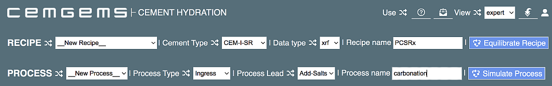
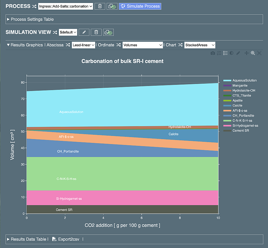
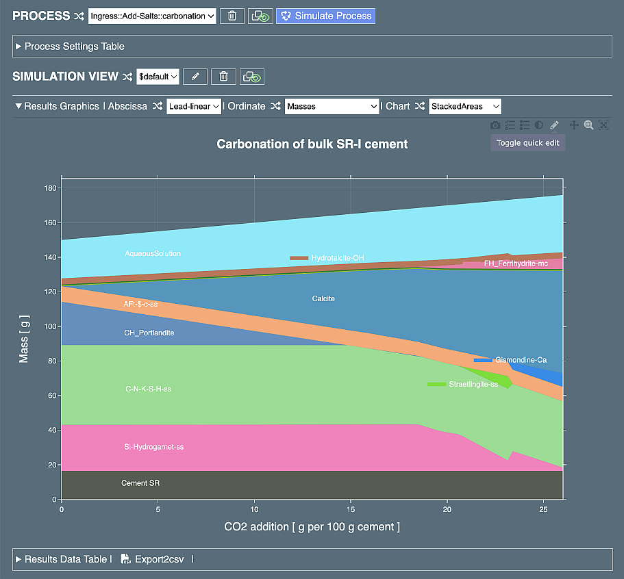
After setting these selections and entering Recipe name and Process name, click on the "Simulate process" button to equilibrate the parent recipe, simulate process, and plot the simulation results. In the Plot Select row, change Abscissa to "Lead-linear" and Ordinate to "Volumes" to see the plot frame below:
The "Ingress::Add-Salts" template defines a linear process with a stepwise addition of the mass (g) of "Salts" material (to mimick the in-diffusion of ions) and compensating removal of CaO (to depict the out-diffusion of Ca+2 and OH- ions). All template recipes by default define the "Salts" material as composed of 100 %mass CO2 constituent, hence, the "Ingress:Add-Salts:" will simulate the carbonation process (an addition of 0 to 10 g CO2 in 101 steps). To simulate the ingress of another salt, the parent recipe needs to be cloned and the composition of "Salts" material needs to be modified.
In this tutorial page, we will look at what can be modified directly in the (cloned) process definition document. A look at the above plot tells us that a more complete qualitative picture of cement carbonation can be obtained when the simulation is performed in a broader interval of CO2 additions, namely 101 steps by adding 0 to 26 g CO2.
Modifying process definition in Process Settings Table
Now, find the Process Settings Table and (by clicking on triangles) expand it as shown below:
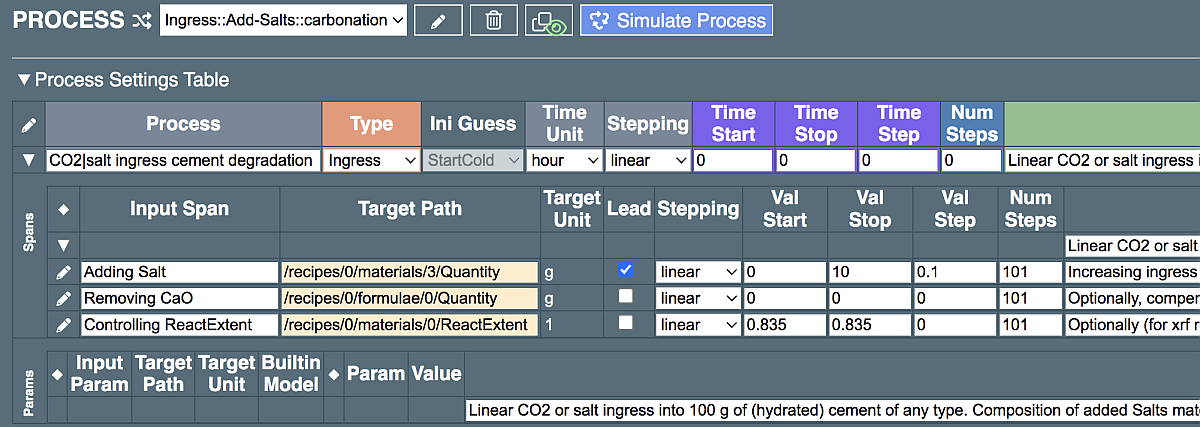
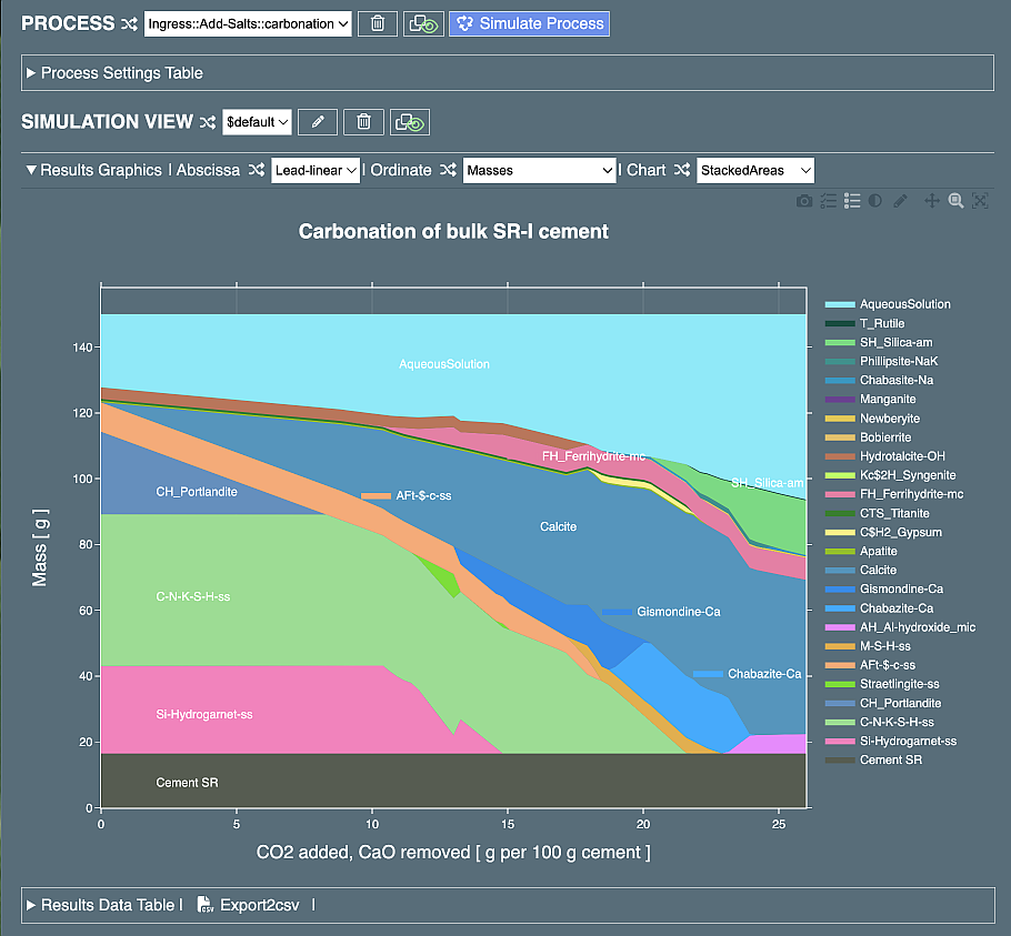
It is seen that this process does not depend on time; the Params subtable is empty; and the Spans subtable contains three input spans. The first (leading) span "Adding Salt" actually targets Quantity of "CO2" constituent in "Salts" material that changes from ValStart = 0 to ValStop = 10 with step 0.1 (all in g) in 101 steps. The second span "Removing CaO" sets zero addition of CaO at all steps, and the third span keeps ReactExtent (degree of reaction, DoR) of "Cement" material constant at 0.835.
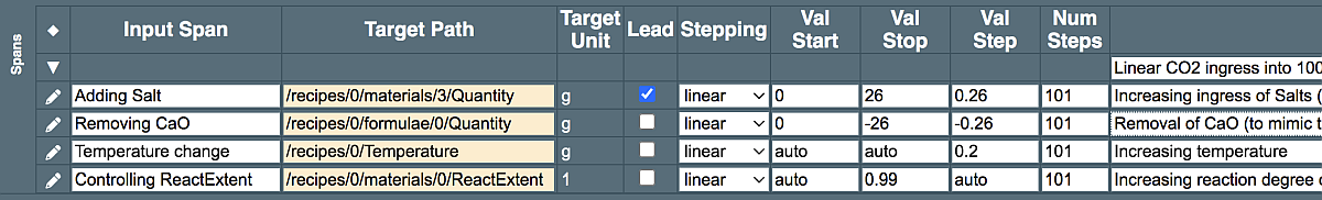
To expand the interval of "Adding Salt" for the maximum addition of 26 g CO2, replace 10 with 26 in the ValStop cell, and 0.1 with a word "auto" in the ValStep cell (the step increment will be calculated automatically). Now the Spans subtable should look like this below:
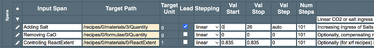
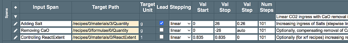
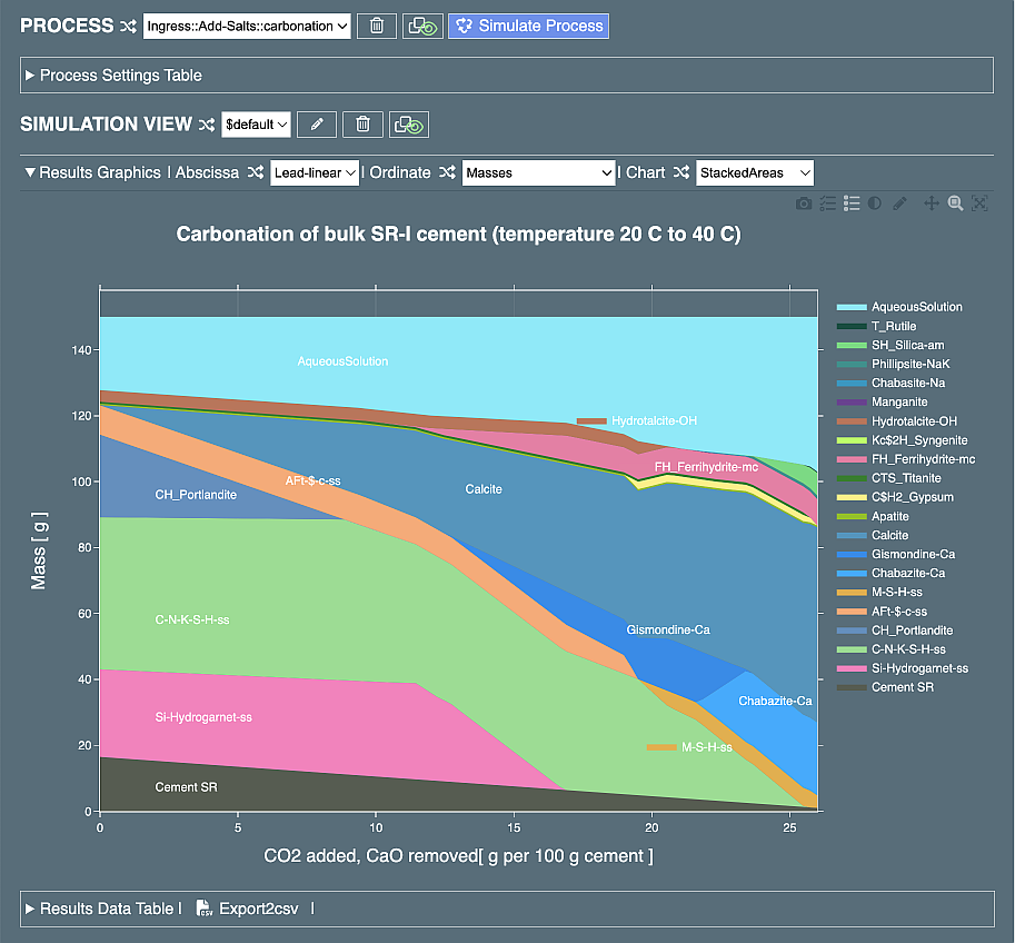
Click on "Simulate Process" button to re-run the process , save it and plot the results. Select "Masses" option in the "Ordinate" above the plot, which then should look like this:
The carbonation profile is now more advanced, with portlandite and siliceous hydrogarnet disappearing,a lot of calcite produced, but C-S-H phase still present in significant amounts. This profile may qualitatively resemble the advanced carbonation of concrete or mortar on air, where in-diffusion of CO2 and H2O is possible, but out-diffusion of Ca is not possible, as it would be during the carbonation process in water. We can easily modify this process definition to check what will change in this "under-water" carbonation case: go back to the Spans subtable and modify it as shown below.
For simplicity, here is assumed that the same mass of CaO is removed at each step as the mass of CO2 added. Re-simulating the process should yield the new plot as shown:
It is clear that in this hypothetical edge case, the carbonation proceeds completely, until all the calcium is converted into calcite, and all the C-S-H - into the amorphous silica phase. The mass of the system stays constant. By re-plotting with other ordinates, you can see the dramatic changes in solubilities of many elements, and a decrease in pH from 13 down to 6 or so, as the excess CaO is removed from the system. Back to the above plot, we recognise that the amount of residual (unreacted) Cement SR clinker remains constant (a gray area at the bottom) at the level set in the parent recipe (28 days). This is not a too realistic scenario because in the real world, cement carbonation (or ingress of any other ions) is a slow process controlled by diffusion. So, a more realistic scenario would be to allow the residual clinker slowly react more and more along with the carbonation progress. Fortunately, this more realistic (still qualitative) scenario is easy to implement by modifying the third span. By adding one more span, a linear change in temperature or in w/b ratio can be set up, for instance.
The first look at a process document in jsoneditor
To get access to the whole process JSON document, click on the "Edit JSON data" button (a pencil inside of a rectangle) in table header to the left of "Process". This will open the jsoneditor widget. By scrolling and clicking on triangles, expand the rows until you see entries in the inputSpans list. This list has three entries (spans); we have already modified the first two spans. Using the small menu icon to the left of a list entry, you can duplicate or remove this entry:
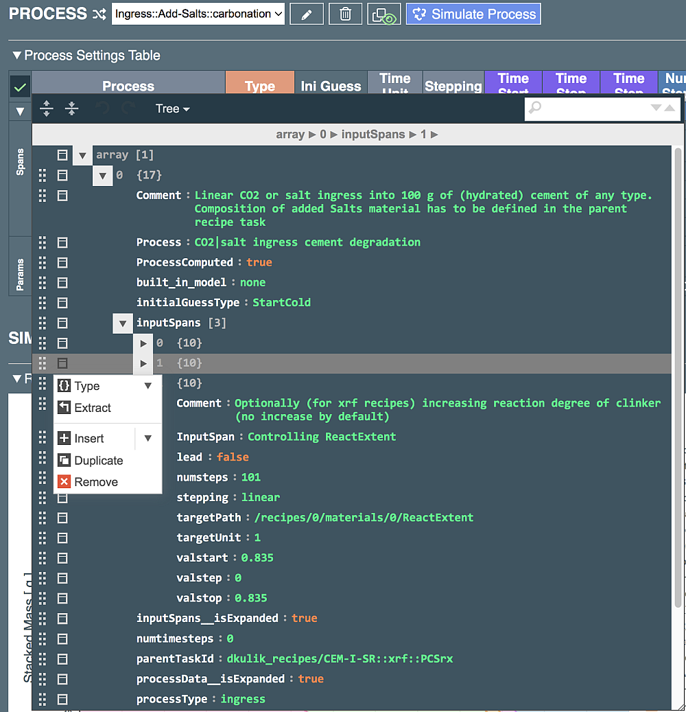
After duplicating the list entry in order to add one more way of change of the recipe inputs in the process simulation, close the jsoneditor by clicking on the green tick in its upper left corner, then expand the Process Settings Table again in order to edit the duplicated entry to make it operational. For that, find the duplicated entry (now the third one) in the Spans subtable.
The "Target Path" field contains a string (JSON path) showing which field of the current recipe input will be changed. In this case, the Quantity of FOrmula #0 in Recipe #0. Note that this field (and its units, "g") can be seen by expanding the input recipe in the "Inputs" area of the Recipe Inputs Table.
To change the Target Path, double-click on it (with a visible background color change); scroll the web page up to the Recipe Inputs Table (there some cells and columns also show a colored background); find among colored cells the one that will be the target (expand the subtable, if needed), for instance a cell under "Temp" (Temperature) in the Recipe row; and double-click on that target cell (colored background disappears).
Go back to the Process Settings Table to see the new Target Path ("/recipes/0/Temperature"). Edit a cell to the left of the target path to "Temperature change" or similar, and cells to the right - to "auto" "auto" "0.2" "101". This means to take temperature from the initial recipe and increment 0.2 degrees per step, until after 100 steps, the temperature becomes 20 degrees higher.
In the last row "Controlling ReactExtent" of Spans subtable, for a stepwise increase of ReactExtent of "Cement", set the iterator cells to "auto" "0.99" "auto" "101". This means to take reaction extent from that given in the initial recipe and increase it to 0.99 after 100 steps (the increment will be calculated automatically). After everything is edited, the Spans subtable should look as shown below:
Click on the "Simulate Process" button to re-calculate the process. After some seconds, the new plot appears:
This time, it is seen indeed, the mass of residual Cement SR clinker goes down from 15% to 1%, as expected. Hence, C-S-H is not totally exhausted within the CO2 addition interval. The effect of increasing temperature is less evident, can be seen only upon saving and comparing various plots for both constant-temperature and variable-temperature variants. To do this, it would be good to clone the process under the name "carbo-rxt-increase". In the Process row, click on the "Clone" button (squares and a green eye), enter the new process name, and click "Clone". The plot frame disappears. Before starting the simulation, expand the Process Settings Table and modify the "Temperature change" iterator to keep the constant temperature (as it was initially in the process template). Then simulate the cloned process and explore the results.
A large pink field in the left-lower part of the diagram is visible, it belongs to Si-Hydrogarnet-ss (siliceous hydrogarnet solid solution) phase. To explore what happens if Si-Hydrogarnet-ss cannot precipitate, for instance due to kinetic hindrances, open the Phases & Aliases table in the recipe; find Si-Hydrogarnet-ss phase and restrict its amount to 0; then re-run the simulation and observe how the process diagram has changed. In a similar way, you can explore what happens if zeolites (Chabasite-Ca and Chabasite-Na) are allowed to precipitate. In this case, the plot will look like this:
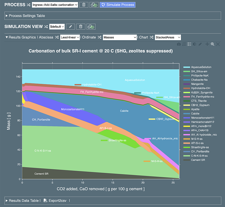
Zeolite (Chabasite-Ca) now appears as a cyan field in the lower-right part of the diagram.
Adjusting parameters in hydration kinetics processes
In CemGEMS, two built-in methods are currently available for simulating cement hydration as function of time:
- (a) Modified Parrot & Killoh (mP&K) model;
- (b) Four-parameter logistic 4PL (5PL) model.
Both models control the reaction extents (degrees) of Cement clinker constituents and/or SCM constituents, but do this in different ways and using different sets of parameters. The time stepping is the same in both models (either linear or log10 time scale in hours). In the current version of CemGEMS, the use of mP&K model is restricted to parent recipes made of ordinary Portland cement (min) templates (with names starting with "CEM-"); the use of 4PL (5PL) logistic model is possible for (min) cement templates of any type.
The parameters and target paths for built-in models are accessible in a separate part of process document, exposed in the Params subtable of the Process Settings Table. In a process definition, the subtable Params (with the respective list) may be present alone or with the Spans subtable and list. The process where built-in hydration models are used must be time-dependent and have valid time iterator values.
To see the time iterators and the Params subtable, and to learn how to work with it, please create a new Recipe of (min) type, for instance, "CEM-II-BV:min:init" and a new process "Hydration-MPK:Time-log:new", and click on the "Simulate Process" button. Then expand the Process Settings Table.
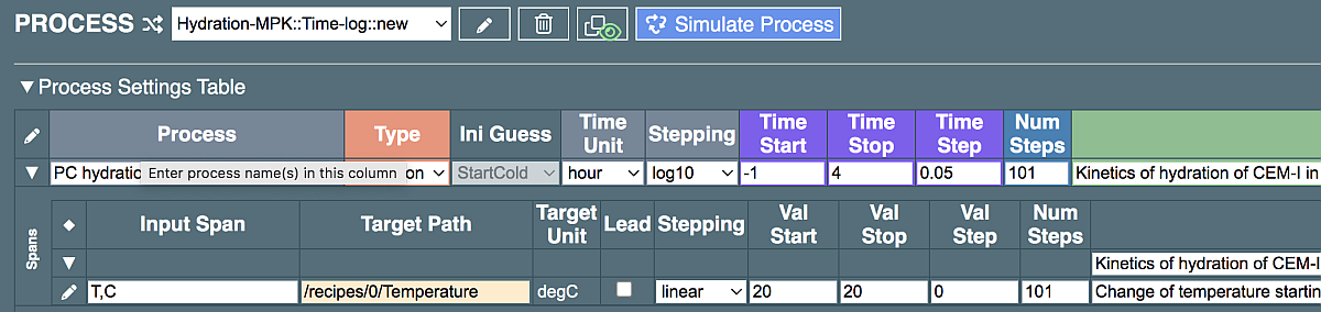
The time span, time stepping, or number of time steps can be easily adjusted in the Process row by tweaking the (string) values in "Time Start", "Time Step", "Time Stop", "Num Steps" columns. If "Time Step" value was changed, the value "auto" can be entered into "Num Steps" field, or vice versa. The "auto" string will be automatically replaced by a consistent number before the process simulation. Note, that, if present, the time span will be leading all other spans and params (i.e. it will set the number of steps in all of them).
There is one row in the Spans subtable with Input Span called "T,C" setting constant temperature of 20 deg.C. This span can be used for setting a different temperature, either constant or changing, or using the jsoneditor to duplicate this span to set up other linear changes, as described above.
(a) The modified Parrot & Killoh model
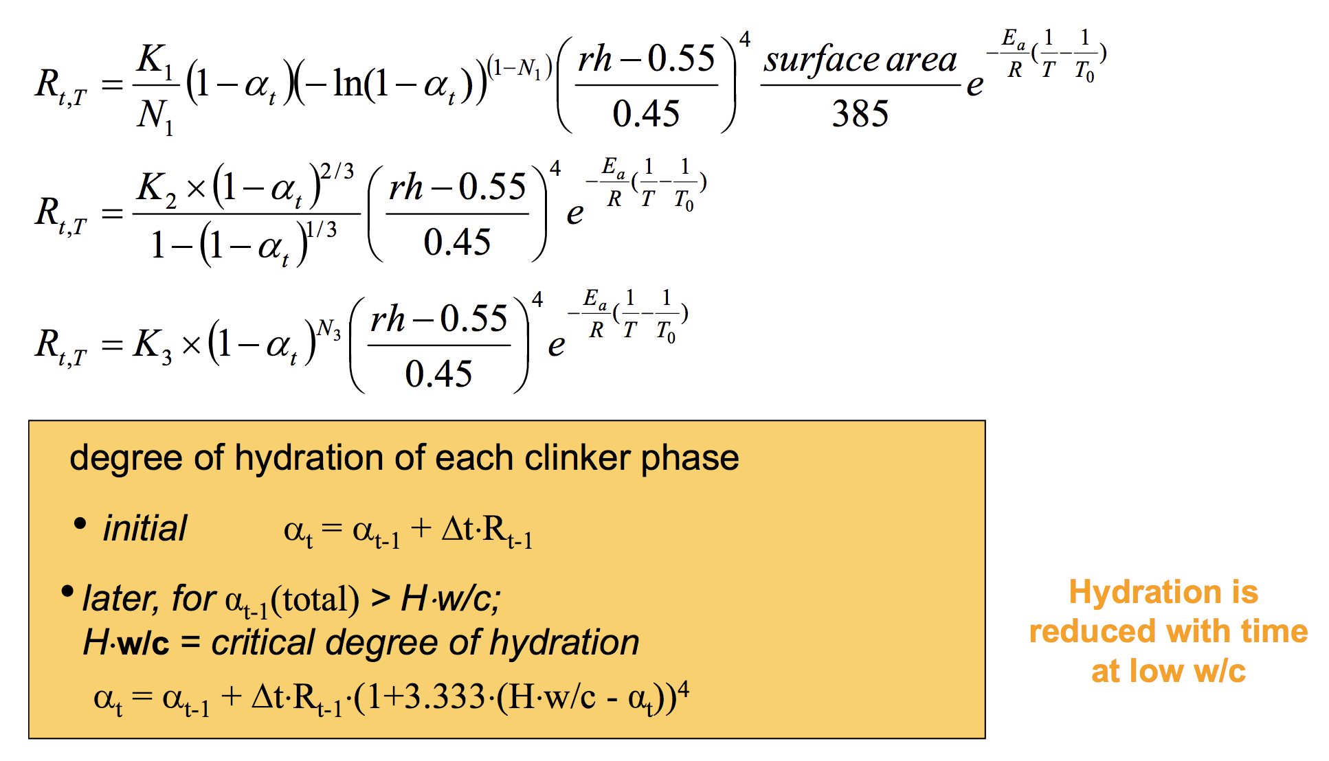
The cement hydration kinetics model of Parrot and Killoh describes the dissolution of clinker constituents (phases) C3S, C2S, C3A, C4AF, with a set of empirical equations for the different rate-controlling mechanisms, including nucleation and growth of hydrated phases, and diffusion of solutes. The dissolution rates at any time by each of these mechanisms depend on the instantaneous degree of hydration alpha(t-1), w/c ratio, and six empirical parameters for each phase. The empirical equations of the modified Parrot and Killoh (mP&K) model are shown below:
From B.Lothenbach @Empa, see also details in this paper:
- Lothenbach, B., Le Saout, G., Gallucci, E., Scrivener, K. (2008) Influence of limestone on the hydration of Portland cements. Cement and Concrete Research, 38(6), 848-860.
The overall rate Rov (1/day, time t in days) used in the last equation above is the minimum of three rates defined by three uppermost equations:
Rov = min( Rng, Rdf, Rhs )
where Rng is the rate of nucleation and growth (of hydrated products) with rate constant K1; Rdf is the rate of diffusion (of dissolved components) with rate constant K2; and Rhs is the rate of secondary products shell formation, with rate constant K3. T is the actual temperature (K) and T0 is the reference temperature (298.15 K). Parameters such as rh (relative humidity), wc (water/binder mass ratio), and specific surface area in m2/kg are obtained from the parent recipe for the process. The values of empirical parameters K1, N1, K2, K3, N3, H, and Ea (activation energy in J/mol) in this order are provided as parameters values in items of Params list of the Hydration-MPK (or Hydration-PK) process templates.
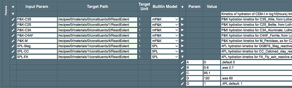
An example of Params subtable with five mP&K parameter sets for main Portland cement constituents (with the one for C2S belite expanded) is shown below:
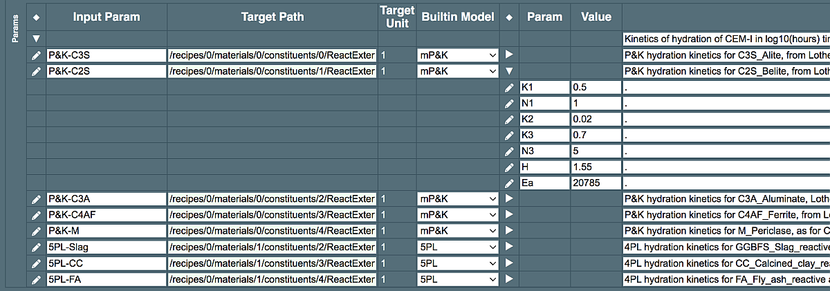
Note that in the array of parameters (columns "Param" and "Value"), the entries (rows) can go in any order because the parameter values are identified by parameter names ("K1", "N1", ...). Any Param row will be ignored if the respective constituent is present in zero Quantity; otherwise, any wrong parameter name or missing parameter row will cause an error during the process simulation. If you modify any parameter value (now taken from process template) then mark this by typing a comment to the right and indicate the reason and the old value of that parameter.
It is important to know that the rates and reaction extents (degrees) in the mP&K model, computed at time t, depend on the rates computed at the previous time step (at time t-1) and on the time step duration dt (hence, dt value should not be too large). This is in contrast with the 4PL/5PL model, where the reaction extent only depends on the current value of time t and not on any previous history of the simulation.
(b) The 5PL (4PL) logistic function model
This is a simple empirical model used in cement chemistry for calculating the degree of hydration (reaction extent) of clinker or SCM materials or constituents alpha(t) at time t (in days). The full 5PL (5-parameter logistic) function is
alpha(t) = D+((A-D)/(1.0+((t/C)^B)))^G
where alpha(t) is in %% of the material reacted at time t, and the parameters (in order of appearance in process span parameters value list) are
| Parameter | Explanation | Interval | Comment |
|---|---|---|---|
| A | minimum asymptote at zero time, %% | 0 <= A < 100 | usually 0 |
| B | steepness of the sigmoid curve slope | ||
| C | time position of inflection point, days | C > 0 | |
| D | maximum asymptote at infinite time, %% | A < D < 100 | |
| G | skew (asymmetry) parameter | 0.1 <= G <= 5.0 | G=1 reduces to 4PL model |
As CemGEMS Process simulator uses time in hours and ReactExtent in unit fraction scale (0 < ReactExtent < 1), the time t and alpha(t) are rescaled accordingly to use equation (5PL) with parameters in scales typical for cement literature.
The above equation (4PL or 5PL) describes a sigmoidal curve that starts at the minimum asymptote, increases rather steeply at some defined slope in the middle, and levels off to the maximum asymptote, optionally with some skew to either side. In applications to cement hydration, these parameters are usually regressed from XRD measurements of how the amounts of clinker minerals or SCMs change with time. In comparison with the mP&K hydration kinetics model, actually applicable to Portland cements only, the 4PL or 5PL equation can be used for any cement hydration process, provided that the empirical XRD data on the evolution of volume or mass of anhydrous minerals or SCM constituents are available. However, the logistic function model is purely empirical and has no internal controls for changing temperature, relative humidity, specific surface area, and other factors.
An example of the Params subtable with three 5PL parameter sets for some common SCM constituents (with the one for Fly Ash expanded) is shown below:
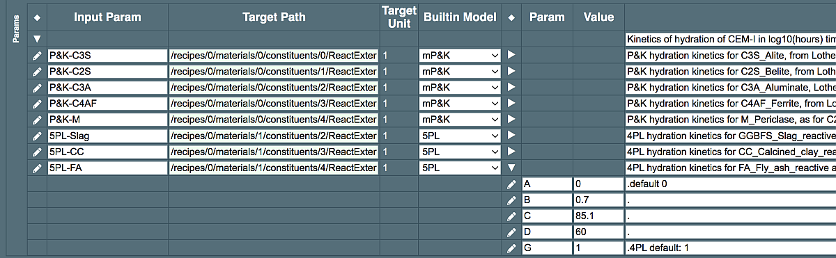
As for the mP&K model, in the array of parameters (columns "Param" and "Value"), the entries (rows) can follow in any order because the parameter values are identified by parameter names ("A", "B", ...). Any Param row will be ignored if the respective constituent is present in zero Quantity; otherwise, any wrong parameter name or missing parameter row will cause an error during the process simulation. If you modify any parameter value (now taken from process template) then mark this by typing a comment to the right and indicate the reason and the old value of that parameter.
More about the 4PL and 5PL logistic (sigmoidal) functions can be found in this paper:
- Gottschalk, P.G., Dunn, J.R. (2005). The five-parameter logistic: A characterization and comparison with the four-parameter logistic. Analytical Biochemistry 343, 54–65.
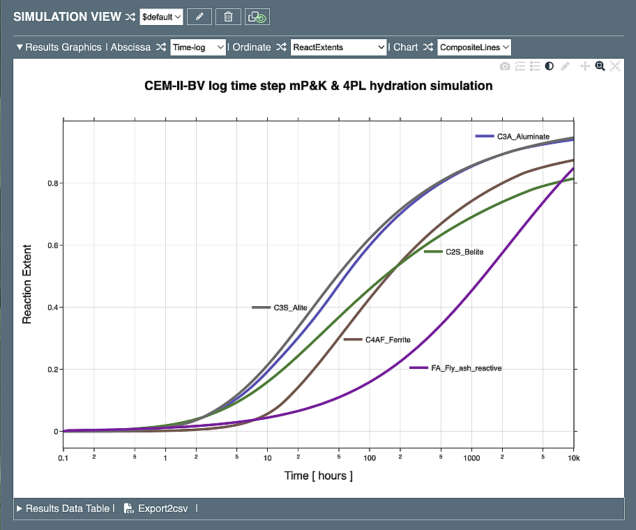
The simulation of the "Hydration-MPK:Time-log:new" process based on the "CEM-II-BV:min:init" recipe results in the following diagrams: one
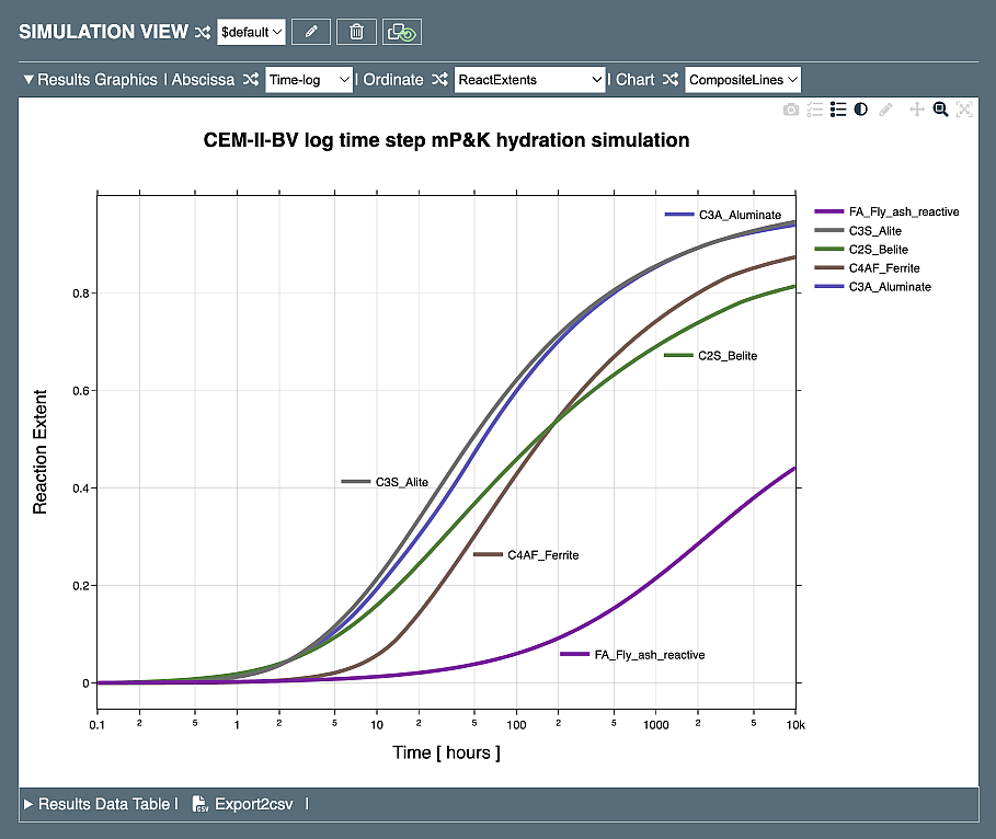
showing the evolution of reaction extents (DoR) of clinker constituents and fly ash SCM computed in logarithmic time scale, and another
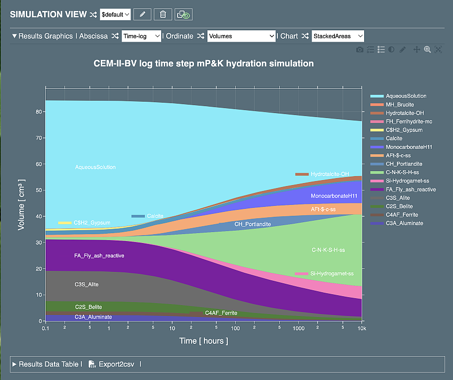
showing how the volumes of phases, residual constituents and SCMs change with time upon hydration. As discussed below, it is actually very easy to control and modify such (blended) cement hydration simulations.
Adjusting Modified Parrot & Killoh (mP&K) model
After creating or cloning and simulating the 'Hydration-MPK' process, you can open the process definition document in Process Settings Table (expand the table and the Params subtable, as shown above). The first Param row in the list changes the ReactExtent input value of the C3S (alite) constituent of Cement material in the recipe, as addressed in the 'Target Path' string. The indexes used in this string (all zeros in the snippet) correspond to those in the parent recipe of the process. For example, in the second Param row, belite C2S is addressed as follows:
/recipes/0/materials/0/constituents/1/ReactExtent
Target Path in the Param row works in the same way as the Target Path in the Span lost row (see above). To change the Target Path, double-click on it (with a visible background color change); scroll the web page up to the Recipe Inputs Table (there some cells and columns also show a colored background); find among colored cells the one that will be the target (expand the subtable, if needed), for instance a cell under "ReactExt" in the Material 'Cement' constituent 'Belite'row; and double-click on that target cell (colored background disappears).
Go back to the Process Settings Table to see the new Target Path ("/recipes/0/materials/0/constituents/1/ReactExtent"). The actual value of the target data at each process step is computed by a built-in subroutine of CemGEMS backend GEMSW code, according to the 'Builtin Model' code and the list of 'Param' and 'Value'. Here, you can change any of parameter values, if necessary. The value ranges and units of measurements correspond to the description in the paper cited in the 'source' field, except the last one - the activation energy - provided later by Prof. B. Lothenbach.
Params subtable rows can be duplicated or deleted using jsoneditor as described above for the rows of Spans subtable. Keep in mind that during process simulation, any Params row (and its target) will be ignored if the respective Constituent, Material or Formula has Quantity equal to zero.
Adjusting empirical 4PL (5PL) logistic function model
The only difference between Params rows for mP&K and 5PL models is different lists of parameter names and their values. Otherwise, the target paths and the modification of ReactExt fields are performed in the same way. The value ranges correspond to the description in the paper cited in the 'source' field, except the last G parameter that expands the 4PL model into the 5PL one, if set to a value different from 1.0. Keep in mind that 5PL parameters are purely empirical, they contain no correction on temperature, relative humidity, specific surface area etc. that the mP&K model has. Nevertheless, the mP&K model is not applicable to SCMs and even constituents of CSA cements, in which cases, the 4PL or 5PL fits to QXRD data are commonly used.
It is relatively easy to adjust the 5PL parameters. For example, let us explore what happens with the hydration profile if the FA (fly ash) SCM will react much faster. In the Params subtable, expand the last row for FA to see 5PL parameters, and increase the 'A' and 'D' parameters as shown below:
Now run the process simulation again, then select the "ReactExtents" plot:
Compared to the initial case, the reaction extent (DoR) of FA (fly ash) increases earlier and to much higher percentage. Examining the volumes of phases:
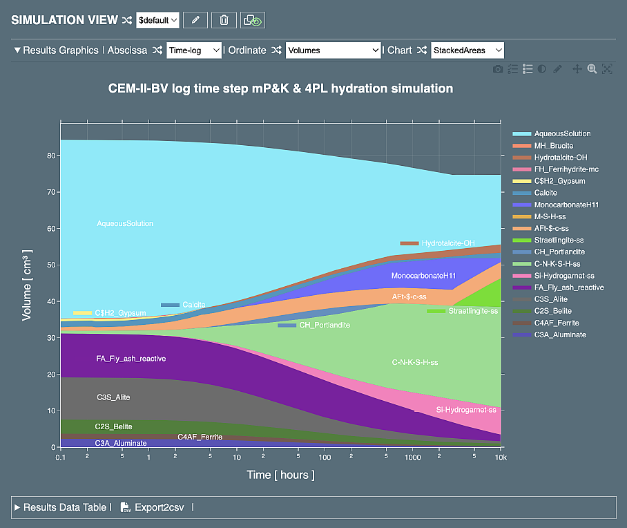
shows that the amount of residual fly ash decreases earlier, portlandite is consumed faster, more siliceous hydrogarnet is formed at longer times, and straetlingite starts to form at cost of monocarbonate. We see indeed that this kind of controlling the process simulation of cement hydration is relatively easy.